目錄
- 概述
- 導包
- 數據讀取
- 數據預處理
- 構建網絡模型
- 數據可視化
- 完整代碼
概述
具體的案例描述在此就不多贅述. 同一數據集我們在機器學習里的隨機森林模型中已經討論過.
導包
import numpy as np
import pandas as pd
import datetime
import matplotlib.pyplot as plt
from pandas.plotting import register_matplotlib_converters
from sklearn.preprocessing import StandardScaler
import torch
數據讀取
# ------------------1. 數據讀取------------------

# 讀取數據
data = pd.read_csv("temps.csv")

# 看看數據長什么樣子
print(data.head())

# 查看數據維度
print("數據維度:", data.shape)

# 產看數據類型
print("數據類型:", type(data))
輸出結果:
year month day week temp_2 temp_1 average actual friend
0 2016 1 1 Fri 45 45 45.6 45 29
1 2016 1 2 Sat 44 45 45.7 44 61
2 2016 1 3 Sun 45 44 45.8 41 56
3 2016 1 4 Mon 44 41 45.9 40 53
4 2016 1 5 Tues 41 40 46.0 44 41
數據維度: (348, 9)
數據類型: class 'pandas.core.frame.DataFrame'>
數據預處理
# ------------------2. 數據預處理------------------

# datetime 格式
dates = pd.PeriodIndex(year=data["year"], month=data["month"], day=data["day"], freq="D").astype(str)
dates = [datetime.datetime.strptime(date, "%Y-%m-%d") for date in dates]
print(dates[:5])

# 編碼轉換
data = pd.get_dummies(data)
print(data.head())

# 畫圖
plt.style.use("fivethirtyeight")
register_matplotlib_converters()

# 標簽
labels = np.array(data["actual"])

# 取消標簽
data = data.drop(["actual"], axis= 1)
print(data.head())

# 保存一下列名
feature_list = list(data.columns)

# 格式轉換
data_new = np.array(data)

data_new  = StandardScaler().fit_transform(data_new)
print(data_new[:5])
輸出結果:
[datetime.datetime(2016, 1, 1, 0, 0), datetime.datetime(2016, 1, 2, 0, 0), datetime.datetime(2016, 1, 3, 0, 0), datetime.datetime(2016, 1, 4, 0, 0), datetime.datetime(2016, 1, 5, 0, 0)]
year month day temp_2 ... week_Sun week_Thurs week_Tues week_Wed
0 2016 1 1 45 ... 0 0 0 0
1 2016 1 2 44 ... 0 0 0 0
2 2016 1 3 45 ... 1 0 0 0
3 2016 1 4 44 ... 0 0 0 0
4 2016 1 5 41 ... 0 0 1 0
[5 rows x 15 columns]
year month day temp_2 ... week_Sun week_Thurs week_Tues week_Wed
0 2016 1 1 45 ... 0 0 0 0
1 2016 1 2 44 ... 0 0 0 0
2 2016 1 3 45 ... 1 0 0 0
3 2016 1 4 44 ... 0 0 0 0
4 2016 1 5 41 ... 0 0 1 0
[5 rows x 14 columns]
[[ 0. -1.5678393 -1.65682171 -1.48452388 -1.49443549 -1.3470703
-1.98891668 2.44131112 -0.40482045 -0.40961596 -0.40482045 -0.40482045
-0.41913682 -0.40482045]
[ 0. -1.5678393 -1.54267126 -1.56929813 -1.49443549 -1.33755752
0.06187741 -0.40961596 -0.40482045 2.44131112 -0.40482045 -0.40482045
-0.41913682 -0.40482045]
[ 0. -1.5678393 -1.4285208 -1.48452388 -1.57953835 -1.32804474
-0.25855917 -0.40961596 -0.40482045 -0.40961596 2.47023092 -0.40482045
-0.41913682 -0.40482045]
[ 0. -1.5678393 -1.31437034 -1.56929813 -1.83484692 -1.31853195
-0.45082111 -0.40961596 2.47023092 -0.40961596 -0.40482045 -0.40482045
-0.41913682 -0.40482045]
[ 0. -1.5678393 -1.20021989 -1.8236209 -1.91994977 -1.30901917
-1.2198689 -0.40961596 -0.40482045 -0.40961596 -0.40482045 -0.40482045
2.38585576 -0.40482045]]
構建網絡模型
# ------------------3. 構建網絡模型------------------

x = torch.tensor(data_new)
y = torch.tensor(labels)

# 權重參數初始化
weights1 = torch.randn((14,128), dtype=float, requires_grad= True)
biases1 = torch.randn(128, dtype=float, requires_grad= True)
weights2 = torch.randn((128,1), dtype=float, requires_grad= True)
biases2 = torch.randn(1, dtype=float, requires_grad= True)

learning_rate = 0.001
losses = []

for i in range(1000):
    # 計算隱層
    hidden = x.mm(weights1) + biases1
    # 加入激活函數
    hidden = torch.relu(hidden)
    # 預測結果
    predictions = hidden.mm(weights2) + biases2
    # 計算損失
    loss = torch.mean((predictions - y) ** 2)

    # 打印損失值
    if i % 100 == 0:
        print("loss:", loss)
    # 反向傳播計算
    loss.backward()

    # 更新參數
    weights1.data.add_(-learning_rate * weights1.grad.data)
    biases1.data.add_(-learning_rate * biases1.grad.data)
    weights2.data.add_(-learning_rate * weights2.grad.data)
    biases2.data.add_(-learning_rate * biases2.grad.data)

    # 每次迭代清空
    weights1.grad.data.zero_()
    biases1.grad.data.zero_()
    weights2.grad.data.zero_()
    biases2.grad.data.zero_()
輸出結果:
loss: tensor(4746.8598, dtype=torch.float64, grad_fn=MeanBackward0>)
loss: tensor(156.5691, dtype=torch.float64, grad_fn=MeanBackward0>)
loss: tensor(148.9419, dtype=torch.float64, grad_fn=MeanBackward0>)
loss: tensor(146.1035, dtype=torch.float64, grad_fn=MeanBackward0>)
loss: tensor(144.5652, dtype=torch.float64, grad_fn=MeanBackward0>)
loss: tensor(143.5376, dtype=torch.float64, grad_fn=MeanBackward0>)
loss: tensor(142.7823, dtype=torch.float64, grad_fn=MeanBackward0>)
loss: tensor(142.2151, dtype=torch.float64, grad_fn=MeanBackward0>)
loss: tensor(141.7770, dtype=torch.float64, grad_fn=MeanBackward0>)
loss: tensor(141.4294, dtype=torch.float64, grad_fn=MeanBackward0>)
數據可視化
# ------------------4. 數據可視化------------------
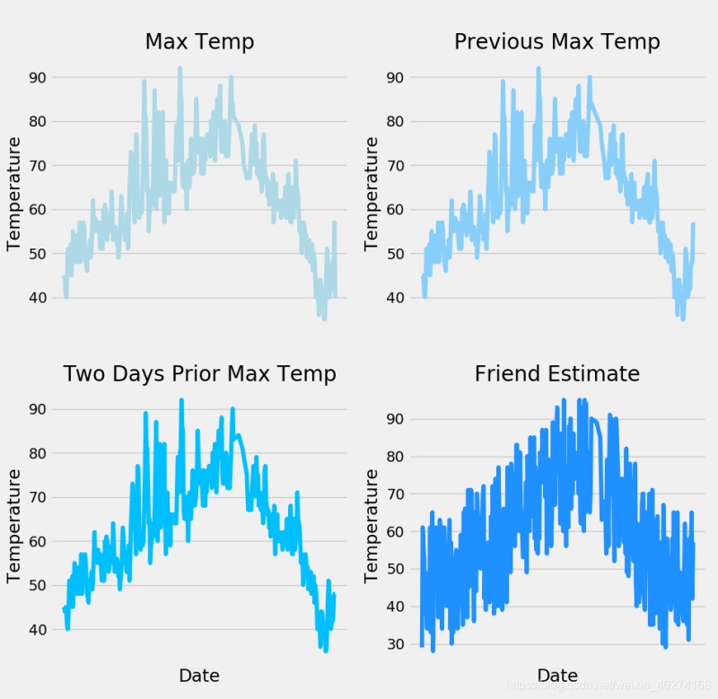
def graph1():
# 創建子圖
f, ax = plt.subplots(2, 2, figsize=(10, 10))
# 標簽值
ax[0, 0].plot(dates, labels, color="#ADD8E6")
ax[0, 0].set_xticks([""])
ax[0, 0].set_ylabel("Temperature")
ax[0, 0].set_title("Max Temp")
# 昨天
ax[0, 1].plot(dates, data["temp_1"], color="#87CEFA")
ax[0, 1].set_xticks([""])
ax[0, 1].set_ylabel("Temperature")
ax[0, 1].set_title("Previous Max Temp")
# 前天
ax[1, 0].plot(dates, data["temp_2"], color="#00BFFF")
ax[1, 0].set_xticks([""])
ax[1, 0].set_xlabel("Date")
ax[1, 0].set_ylabel("Temperature")
ax[1, 0].set_title("Two Days Prior Max Temp")
# 朋友
ax[1, 1].plot(dates, data["friend"], color="#1E90FF")
ax[1, 1].set_xticks([""])
ax[1, 1].set_xlabel("Date")
ax[1, 1].set_ylabel("Temperature")
ax[1, 1].set_title("Friend Estimate")
plt.show()
輸出結果:
完整代碼
import numpy as np
import pandas as pd
import datetime
import matplotlib.pyplot as plt
from pandas.plotting import register_matplotlib_converters
from sklearn.preprocessing import StandardScaler
import torch


# ------------------1. 數據讀取------------------

# 讀取數據
data = pd.read_csv("temps.csv")

# 看看數據長什么樣子
print(data.head())

# 查看數據維度
print("數據維度:", data.shape)

# 產看數據類型
print("數據類型:", type(data))

# ------------------2. 數據預處理------------------

# datetime 格式
dates = pd.PeriodIndex(year=data["year"], month=data["month"], day=data["day"], freq="D").astype(str)
dates = [datetime.datetime.strptime(date, "%Y-%m-%d") for date in dates]
print(dates[:5])

# 編碼轉換
data = pd.get_dummies(data)
print(data.head())

# 畫圖
plt.style.use("fivethirtyeight")
register_matplotlib_converters()

# 標簽
labels = np.array(data["actual"])

# 取消標簽
data = data.drop(["actual"], axis= 1)
print(data.head())

# 保存一下列名
feature_list = list(data.columns)

# 格式轉換
data_new = np.array(data)

data_new  = StandardScaler().fit_transform(data_new)
print(data_new[:5])

# ------------------3. 構建網絡模型------------------

x = torch.tensor(data_new)
y = torch.tensor(labels)

# 權重參數初始化
weights1 = torch.randn((14,128), dtype=float, requires_grad= True)
biases1 = torch.randn(128, dtype=float, requires_grad= True)
weights2 = torch.randn((128,1), dtype=float, requires_grad= True)
biases2 = torch.randn(1, dtype=float, requires_grad= True)

learning_rate = 0.001
losses = []

for i in range(1000):
    # 計算隱層
    hidden = x.mm(weights1) + biases1
    # 加入激活函數
    hidden = torch.relu(hidden)
    # 預測結果
    predictions = hidden.mm(weights2) + biases2
    # 計算損失
    loss = torch.mean((predictions - y) ** 2)

    # 打印損失值
    if i % 100 == 0:
        print("loss:", loss)
    # 反向傳播計算
    loss.backward()

    # 更新參數
    weights1.data.add_(-learning_rate * weights1.grad.data)
    biases1.data.add_(-learning_rate * biases1.grad.data)
    weights2.data.add_(-learning_rate * weights2.grad.data)
    biases2.data.add_(-learning_rate * biases2.grad.data)

    # 每次迭代清空
    weights1.grad.data.zero_()
    biases1.grad.data.zero_()
    weights2.grad.data.zero_()
    biases2.grad.data.zero_()

# ------------------4. 數據可視化------------------

def graph1():
    # 創建子圖
    f, ax = plt.subplots(2, 2, figsize=(10, 10))

    # 標簽值
    ax[0, 0].plot(dates, labels, color="#ADD8E6")
    ax[0, 0].set_xticks([""])
    ax[0, 0].set_ylabel("Temperature")
    ax[0, 0].set_title("Max Temp")

    # 昨天
    ax[0, 1].plot(dates, data["temp_1"], color="#87CEFA")
    ax[0, 1].set_xticks([""])
    ax[0, 1].set_ylabel("Temperature")
    ax[0, 1].set_title("Previous Max Temp")

    # 前天
    ax[1, 0].plot(dates, data["temp_2"], color="#00BFFF")
    ax[1, 0].set_xticks([""])
    ax[1, 0].set_xlabel("Date")
    ax[1, 0].set_ylabel("Temperature")
    ax[1, 0].set_title("Two Days Prior Max Temp")

    # 朋友
    ax[1, 1].plot(dates, data["friend"], color="#1E90FF")
    ax[1, 1].set_xticks([""])
    ax[1, 1].set_xlabel("Date")
    ax[1, 1].set_ylabel("Temperature")
    ax[1, 1].set_title("Friend Estimate")

    plt.show()


if __name__ == "__main__":
    graph1()
到此這篇關于PyTorch一小時掌握之神經網絡氣溫預測篇的文章就介紹到這了,更多相關PyTorch 神經網絡氣溫預測內容請搜索腳本之家以前的文章或繼續瀏覽下面的相關文章希望大家以后多多支持腳本之家!
您可能感興趣的文章:- PyTorch一小時掌握之autograd機制篇
- PyTorch一小時掌握之神經網絡分類篇
- PyTorch一小時掌握之圖像識別實戰篇
- PyTorch一小時掌握之基本操作篇